What is Dynamic Programming?
Dynamic Programming is the process of simplifying a complicated problem by breaking it down into simpler sub-problems in a recursive manner. In computer science, if a problem can be solved optimally by breaking it into sub-problems and then recursively finding the optimal soltions to the sub-problems, then it is said to have optimal structure.
Dynamic Programming != Recursion
Why should we care about Dynamic Programming?
Optimization. Sometimes, executing recursion can involve repetitive computations and require a lot of resources and time to compute, like O(2n) long. Not as long as O(n!), but in terms of growth rates, exponential computations add up very quickly.
When and Where should Dynamic Programming be used?
If you notice that the problem can be broken into much smaller ones and some of these have overlap (eg, requires the computation of previously calculated values). The main goal is to optimize the code by reducing the repetition of values by storing the results of sub-problems, so they do not have to be calculated again.
How is Dynamic Programming applied?
1. Top-Down Approach, aka Memoization
With this approach, the problem is broken down and if the problem is solved already then the saved value is returned, otherwise, the value of the function is memoized. In other words, it will be calculated for the first time, every other time, and the saved value will be called back. Memoization is a great method for computationally expensive programs.
2. Bottom-Up Approach
This is an effective way of avoiding recursion by decreasing the time complexity that recursion builds up (eg, memory cost because of recalculation of the same values). Here, the solutions to small problems are calculated which builds up the solution to the overall problem.
Example Problem, the Fibonacci Sequence
What is the Fibonacci Sequence?
It is when the previous two numbers in a list is the sum of the next number in the sequence.
fib = [1, 1, 2, 3, 5, 8]
If you wanted to write a function for the above sequence it would look like this:
    def fib(n):
        if n == 1 or n == 2:
            # store 1 in a temp variable, don't return it
            result = 1
        else:
            # if n does not equal 1 or 2, return the sum of the two previous Fibonacci #'s instead
            result = fib(n - 1) + fib(n - 2)

        return result
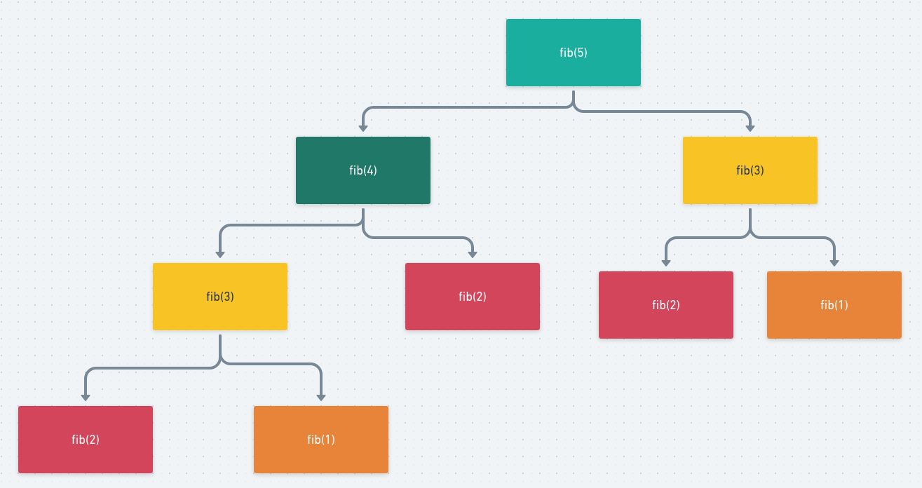
As previously mentioned, this solution is not very effecient because there are computations that we need to repeat over and over again. What do I mean by that? Here’s a visualization.

The red squares represent fib(2) that need to be computed three times, also fib(1) in orange and fib(3) in yellow, each need to be computed twice. No bueno.
Solution, Memoization
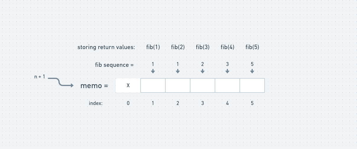
Here’s a break down of implementing memoization for our example problem:
- Use an array whose length is n + 1
- Store the return value for the function of fib of n at the index, n
- Store fib(1) at index 1, fib(2) at index 2, etc…

    def fib(n, memo):
        if memo[n] != null:
            return memo[n]
        if n <= 1:
            return n
        else:
            res = fib(n - 1) + fib(n + 1)
            memo[n] = res
            return res
Solution, Bottom-Up
This approach down not use recursion at all. We created an empty list of length (n + 1) and set the base case of f(0) and f(1) at index positions 0 and 1. This list is created to store the corresponiding calculated values using a for loop for index values 2 up to n.
    def fib(n):
        if n <= 1:
            return n
        lst = [0] * (n + 1)
        lst[0] = 0
        lst[1] = 1
        for i in range(2, n + 1):
            lst[i] = lst[i - 1] + lst[i - 2]
        return lst[n]
As you can see Dynamic Programming is very efficient for optimizing code. It is simple and easy to understand, however it will take practice to fully grasp its utilization.
Shout out to Aleksandra Boguslawska for the great pic!